Throughout the paper, we use the example of the dining philosophers to illustrate the workbench and toolchain. Due to space constraints, the presentation is limited to a few select features of both. Here, we aim to cover the example in more detail by providing additional code snippets, graphs from the Scoop-GTS.

Note that some of the text here is copied verbatim from the paper, however, we will not further indicate those sections here.

SCOOP Implementation

The following SCOOP code implements the dining philosophers as presented in the paper.

The main application that initializes problem instance is implemented in the class APPLICATION:

class
    APPLICATION

create
    make

feature -- Initialisation

    i: INTEGER
    first_fork, left_fork, right_fork: separate FORK
    a_philosopher: separate PHILOSOPHER

    make
            -- Create philosophers and forks
            -- and initiate the dinner.
        do
            philosopher_count := 2
            round_count := 1

            -- Dining Philosophers with `philosopher_count' philosophers and `round_count' rounds.

            from
                i := 1
                create first_fork.make
                left_fork := first_fork
            until
                i > philosopher_count
            loop
                if i < philosopher_count then
                    create right_fork.make
                else
                    right_fork := first_fork
                end
                create a_philosopher.make (i, left_fork, right_fork, round_count)
                launch_philosopher (a_philosopher)
                left_fork := right_fork
                i := i + 1
            end
        end

feature {NONE} -- Implementation

    philosopher_count: INTEGER
            -- Number of philosophers.

    round_count: INTEGER
            -- Number of times each philosopher should eat.

    launch_philosopher (philosopher: separate PHILOSOPHER)
            -- Launch a_philosopher.
        do
            philosopher.live
        end

end

The philosophers’ behaviour is implemented in the class PHILOSOPHER:

class
    PHILOSOPHER

create
    make

feature -- Initialisation

    make (philosopher: INTEGER; left, right: separate FORK; round_count: INTEGER)
            -- Initialise with ID of `philosopher', forks `left' and `right', and for `round_count' times to eat.
        require
            valid_id: philosopher > 0
            valid_times_to_eat: round_count > 0
        do
            id := philosopher
            left_fork := left
            right_fork := right
            times_to_eat := round_count
        ensure
            id_set: id = philosopher
            left_fork_set: left_fork = left
            right_fork_set: right_fork = right
            times_to_eat_set: times_to_eat = round_count
        end

feature -- Access

    id: INTEGER
            -- Philosopher's id.

feature -- Measurement

    times_to_eat: INTEGER
            -- How many times does it remain for the philosopher to eat?

feature -- Basic operations

    eat (left, right: separate FORK)
            -- Eat, having acquired `left' and `right' forks.
        do
            -- Eating takes place.
        ensure
            has_eaten: true
        end

    live
        do
            from
            until
                times_to_eat < 1
            loop
                -- Philosopher `Current.id' waiting for forks.
                eat (left_fork, right_fork)
                --bad_eat
                -- Philosopher `Current.id' has eaten.
                times_to_eat := times_to_eat - 1
            end
        end

    bad_eat
            -- Eat, by first picking up `left_fork' (and picking up `right_fork'
            -- in the `pickup_left' call.
        do
            pickup_left (left_fork)
        end

    pickup_left (left: separate FORK)
            -- After having picked up `left', proceed to pick up `right_fork'.
        do
            pickup_right (right_fork)
        end

    pickup_right (right: separate FORK)
            -- Both forks have been acquired at this point.
        do
            -- eating takes place
        end

feature {NONE} -- Access

    left_fork: separate FORK
            -- Left fork used for eating.   

    right_fork: separate FORK
            -- Right fork used for eating.

invariant
    valid_id: id >= 1

end

Finally, the forks are represented as instances of the trivial class FORK; they do not have any logic associated, but are used as separate objects in philosopher arguments. Consequently, the SCOOP runtime will ensure that a fork can be held by a single philosopher at a time. The implementation is as follows:

class
    FORK

create
    make

feature -- Initialisation

    make
        do
        end

end

A SCOOP-Graph program represenatation

In a first step, we translate the source code to start graph, which mainly consists of a collection of control-flow graphs, each representing a method in the source code. For example, the generated control-flow subgraph can be seen in the following figure.

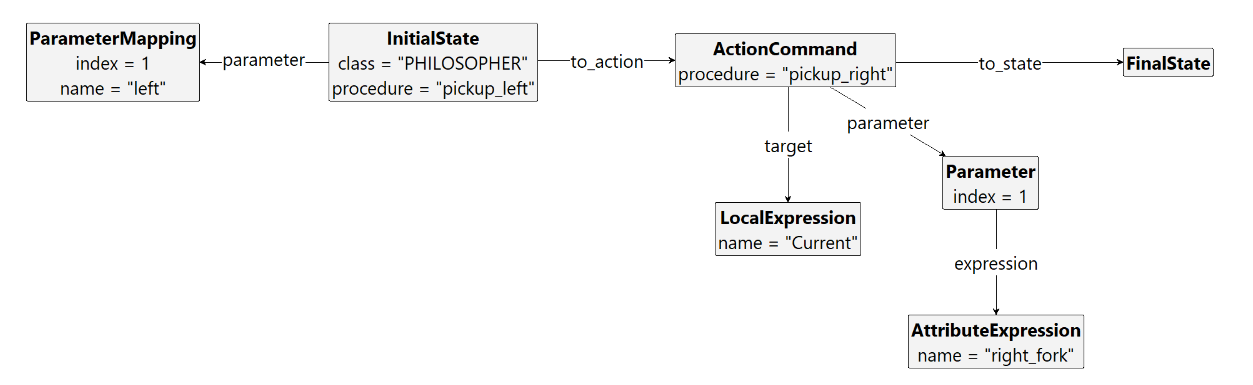
In this example, there are two State nodes (one InitialState and one FinalState node), as well as a single Command node. The ActionCommand corresponds to the source code line Current.pickup_right (right_fork); likewise, other actions such as ActionAssignment or ActionPreconditionTest correspond to the source code abstractions. With this close mapping to the source language, the control-flow-graphs remain easy to understand and intuitive even for SCOOP programmers unfamiliar with graph transformation systems.

Representing runtime state

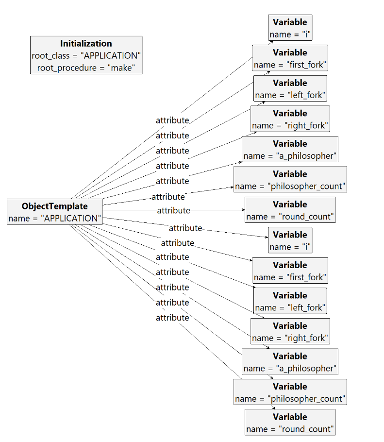
In SCOOP-GTS, there is initally a single node indication the root procedure, i.e., the method that is executed at the beginning of program execution (unlike other languages like C, there is no convention for a program entry point; instead, any method can be selected by instructing the compiler accordingly). Together with Object Templates, i.e., graphs containing class name and attribute names, the runtime state can be initialized. The following figure shows the root configuration node and the template for the APPLICATION class.

In the QoQ semantics, the rule named rule_scoop_qoq_initialize_root is used
to initialize the runtime state representation, shown below.

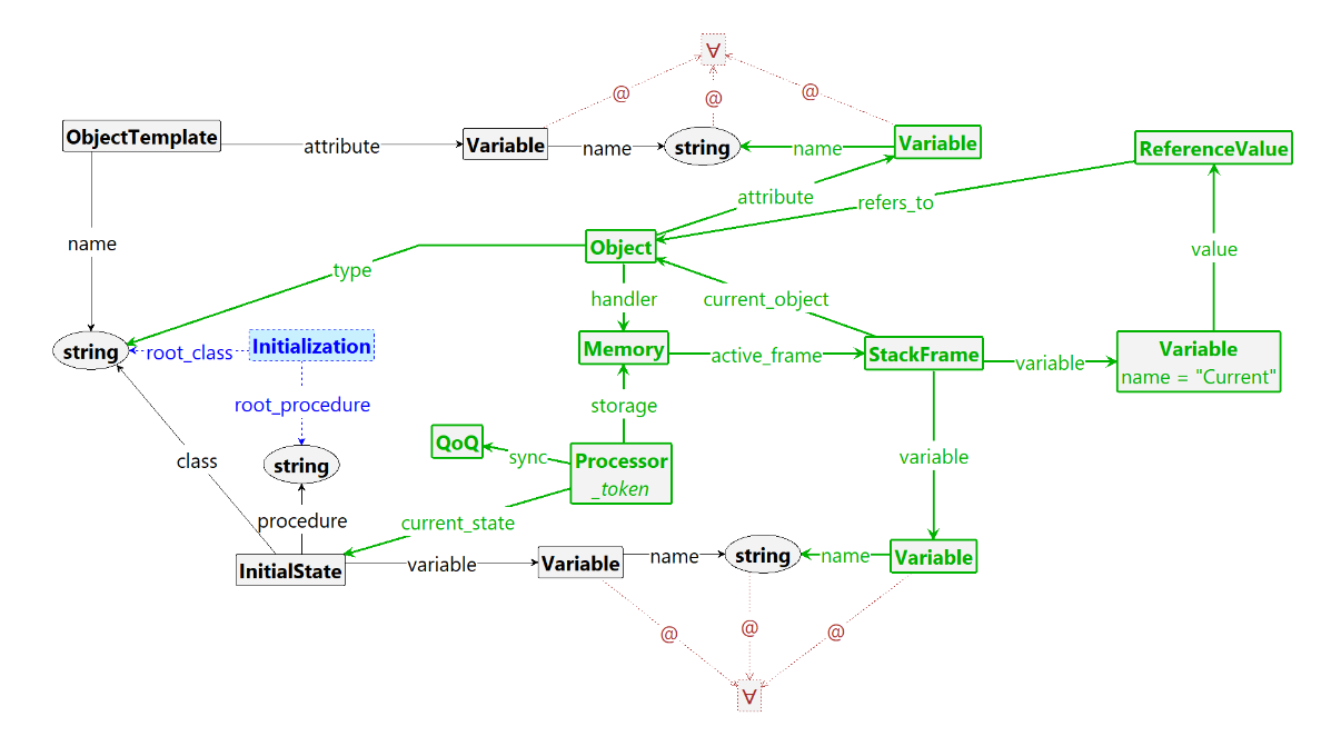
Here, the rule matches the Initialization node which is then deleted upon rule application (indicated by coloring node and edges blue). By matching the root_class edge to the ObjectTemplate with the same name, the rule can create a new Object node (nodes and edges added during application are colored in green). Using a universal quantifier (∀), the rule matches all attributes connected to the template and thus we can create object-local copies. Since this rule is used in the QoQ semantics, the rule also creates the first Processor, as well as a representation of Memory state and an empty queue of queues (QoQ) node. Finally, the processor’s current state is set to the InitialState node of the root procedure.

After this setup, the system is initialized with a root object and a root processor that is about to execute the root procedure. Similar rules exist for the RQ and DSCOOP semantics.

Controlling execution through control programs

The Scoop-Gts consists of a large number of rules (in the source code, each .gpr file corresponds to one rule) in various categories like evaluation of references, cleaning up nodes and edges that are not used anymore, or moving a processor’s execution along the control flow graph. If one simply non-deterministically applies a rule that matches, one has to introduce helper nodes and edges in the graph and rules in order to force a certain execution. For example, a Scheduling node could be introduced to indicate that one of the scheduling rules (such as scoop_qoq_scheduling_action_command_remote_empty, which creates a separate request for a command action) can now be applied. Then, each scheduling rule has a Scheduling node, meaning that only if this node is present the rule can be applied, and each other rule has a negative-application condition for Scheduling, meaning that when the state graph indicates that execution is in the scheduling process, no other rule is applied.

With more and more rules, however, controlling the execution order with (negative) application conditions can be hard to track and results in the introduction of many helper nodes and edges. Furthermore, optimizations that reduce the state space (e.g., by forcing a particular processor the execute local computations as long as possible before handing control to the next processor) are difficult to introduce.

Fortunately, Groove provides so-called control programs, which can be thought of as a set of functions (called recipes) that dictate the order in which rules are applied. A simple example (unrelated to the actual implementation) is as follows:

while (no_error) {
  alap execute_action;
}

recipe execute_action() {
  execute_command_local |
  execute_command_separate |
  ...;
}

Here, the main loop would execute as long as a rule no_error can be applied. In the body, we execute the recipe as long as possible (alap keyword), which in turn applies one of the stated rules nondeterministically (a | b is a nondeterministic choice).

Using control programs helps us to keep rules simple. For example, without control programs, the above rules execute_command_local and execute_command_separate would need to contain application conditions that test whether there is an error or not. With the control program, this can be avoided.

Another advantage is that control programs can be used to force certain interleavings in the state-space where exploring all possibilities is not relevant to the runtime. For example, suppose we have three garbage collection rules that leave the graph in the same state when applied as long as possible. Without a control program, we may end up exploring all different possibilities, just to arrive in the exact same state. In contrast, if we write a control program that applies the rules as long as possible in sequence (that is, alap { first; second; third; }), only a single execution trace is generated.

One major use of the above example in Scoop-Gts is that we can force processors to execute local computations (i.e., computations that do not involve data guarded by other processors) as long as possible before yielding control to the next one. This way, we considerably decrease the branching where it does not matter (in the sense that the asynchronous or distributed behaviour is influenced).

In the case of Scoop-Gts, the control programs are more complex. A simplified version is given in the paper in Listing 5; in the source code, they are stored as .gcp files, and they can be edited in the Groove UI.

Detecting a deadlock

After translating a SCOOP program to a Scoop-Gts graph and selecting the runtime, the Groove Simulator or our command-line wrapper can be used to explore the state space of the program under the selected runtime.

In order to detect discrepancies and errors, we can define rules that are periodically tested during state space exploration. For example, a rule that detects a deadlock involving two processors looks as follows.

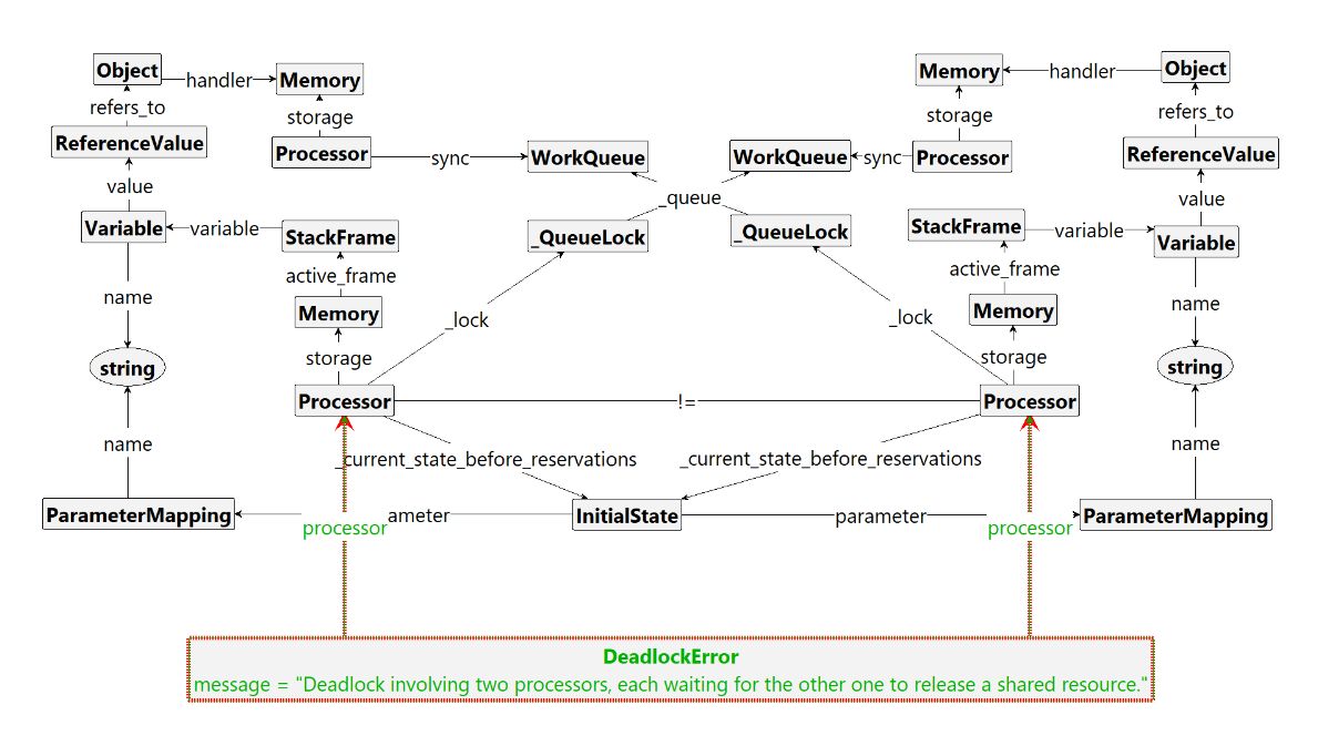
Whenever such a rule matches during state space exploration, this means that under the given semantics, the error may occur. In this example, we then create a DeadlockError node, which is an Error node. Whenever one such node exists, the control program finishes, meaning that such a state is a final state in the generate state space. If there are no errors and execution finishes, final states are graphs where no processor is executing any method anymore, and all that remains are the processor, memory, and queue subgraphs, none of which is connected to a method control-flow graph.

Once the Groove exploration finishes, we can query the final states and inspect them. Since the graphs are saved as simple XML files, we can easily parse and look for Error nodes, such as ErrorDeadlock. If there is such a node, we report it accordingly. While currently not implemented in our tool, the closeness of a Scoop-Gts program representation and the source code, it is straightforward to map errors back to relevant locations in the source code.